This is part 1 of a tutorial series. We recommend following them in order, starting with Part 0: Welcome to ``musica` <0.%20Welcome%20to%20MUSICA.ipynb>`__.

User-Defined Reactions in musica

So far, we’ve created chemical mechanisms using only Arrhenius reactions. Here we’ll introduce a few more, including the powerful “user-defined” reaction. These reaction types give you control over how rate constants are calculated.

We’ll also throw in an Emission and FirstOrderLoss, which actually use the UserDefined type under the hood.

1. Importing Libraries

Below is a list of the required libraries for this tutorial:

import musica
import musica.mechanism_configuration as mc
import matplotlib.pyplot as plt
from scipy.stats import qmc
import pandas as pd
import numpy as np
import seaborn as sns
pd.set_option('display.float_format', str) # This is done to make the arrays more readable
np.set_printoptions(suppress=True) # This is done to make the arrays more readable

2. Base Chemical System

Let’s start with the chemical system we’ve been using in the tutorials to this point, with three species and two reactions.

A = mc.Species(name="A")
B = mc.Species(name="B")
C = mc.Species(name="C")
species = [A, B, C]
gas = mc.Phase(name="gas", species=species)

r1 = mc.Arrhenius(
    name="A_to_B",
    A=4.0e-3,
    C=50,
    reactants=[A],
    products=[B],
    gas_phase=gas
)

r2 = mc.Arrhenius(
    name="B_to_C",
    A=4.0e-3,
    C=50,
    reactants=[B],
    products=[C],
    gas_phase=gas
)

3. Defining User Defined Reactions

This code cell defines three new reactions: one User Defined, one Emission, and one First Order Loss. It then creates a new mechanism containing both the old reactions as well as the three new reactions.

r3 = mc.UserDefined(
    name="complex_rxn",
    scaling_factor=1.0,
    reactants=[A, (B, 2)],
    products=[A, (C, 2), B],
    gas_phase=gas
)

r4 = mc.Emission(
    name="B_emission",
    scaling_factor=1.0,
    products=[B],
    gas_phase=gas
)

r5 = mc.FirstOrderLoss(
    name="C_loss",
    scaling_factor=1.0,
    reactants=[C],
    gas_phase=gas
)

mechanism = mc.Mechanism(
    name="musica_micm_example",
    species=species,
    phases=[gas],
    reactions=[r1, r2, r3, r4, r5]
)

Notice that we don’t specify rate constants for the User-Defined or First-Order Loss reactions, and we don’t specify emission rates. This is because these values can change over time, and unlike standard rate constant types (like Arrhenius reactions), micm doesn’t know how to calculate them based on the current temperature and pressure.

So, it’s our responsibility to calculate these rates and rate constants, and update them in the micm state, as needed.

4. Creating the Solver, State, and Latin Hypercube Sampler

We’ll use the Latin Hypercube Sampler to create the initial conditions, just like in the last tutorial. But, this time around we’ll expand the LHS to eight dimensions: the five original dimensions (temperature, pressure, and concentrations of A, B, and C) and three new dimensions for the User-Defined, Emission, and First-Order Loss reactions.

solver = musica.MICM(mechanism = mechanism, solver_type = musica.SolverType.rosenbrock_standard_order)

num_grid_cells = 100
state = solver.create_state(num_grid_cells)

ndim = 8
nsamples = num_grid_cells

# Create a Latin Hypercube sampler in the unit hypercube
sampler = qmc.LatinHypercube(d=ndim)

# Generate samples
sample = sampler.random(n=nsamples)

# Define bounds for each dimension (temperature, pressure, concentrations of A, B, and C, User-defined reaction, Emission, and Loss)
l_bounds = [275, 100753.3, 0, 0, 0, 0, 0, 0] # Lower bounds
u_bounds = [325, 101753.3, 20, 10, 20, 1, 0.5, 0.5] # Upper bounds

# Scale the samples to the defined bounds
sample_scaled = qmc.scale(sample, l_bounds, u_bounds)

temperatures = sample_scaled[:, 0]
pressures = sample_scaled[:, 1]
concentrations = {
    "A": [],
    "B": [],
    "C": []
}
concentrations["A"] = sample_scaled[:, 2]
concentrations["B"] = sample_scaled[:, 3]
concentrations["C"] = sample_scaled[:, 4]

state.set_conditions(temperatures, pressures)
state.set_concentrations(concentrations)

5. Creating and Setting the User Defined Parameters

The last step in setting the conditions, is providing initial values for our new reactions. To do that, we need to provide them to the state with their unique names. The syntax for the label is PREFIX.reaction-name. The PREFIX is based on the type of reaction:

• USER for User Defined reactions,

• EMIS for Emission reactions, and

• LOSS for First Order Loss reactions.

Then reaction-name is the name we gave to each reaction when it was created (see above).

Once we have the labels, we can use them in a call to the state.set_user_defined_rate_parameters() function to set the values of the reaction rates and rate constants

state.set_user_defined_rate_parameters({
    "USER.complex_rxn": sample_scaled[:, 5],
    "EMIS.B_emission": sample_scaled[:, 6],
    "LOSS.C_loss": sample_scaled[:, 7]
})

6. Solving the System

We’ll solve the system as in previous tutorials, for 600 s in 10 s intervals

concentrations_solved = []
time_step = 10
sim_length = 600
curr_time = 0

while curr_time <= sim_length:
    solver.solve(state, time_step)
    concentrations_solved.append(state.get_concentrations())
    curr_time += time_step
    state.set_user_defined_rate_parameters({
        "EMIS.B_emission": sample_scaled[:, 6] * (1 + 0.5 * np.sin(curr_time / sim_length * 2 * np.pi))
    })

Note how we update the emission rate at each time step. The other two rate constants remain constant throughout the simulation.

7. Visualizing the Results

Now, let’s prepare and plot the results, just like we’ve done before

concentrations_solved_expanded = []
time = []
for i in range(0, sim_length + 1, time_step):
    for j in range(0, num_grid_cells):
        concentrations_solved_expanded.append({key: value[j] for key, value in concentrations_solved[int(i/time_step)].items()})
        time.append(i)
df_expanded = pd.DataFrame(concentrations_solved_expanded)
df_expanded = df_expanded.rename(columns = {'A' : 'CONC.A.mol m-3', 'B' : 'CONC.B.mol m-3', 'C' : 'CONC.C.mol m-3'})
df_expanded['time.s'] = time
df_expanded['ENV.temperature.K'] = np.repeat(temperatures[0], (sim_length/time_step + 1.0) * num_grid_cells)
df_expanded['ENV.pressure.Pa'] = np.repeat(pressures[0], (sim_length/time_step + 1.0) * num_grid_cells)
df_expanded['ENV.air number density.mol m-3'] = np.repeat(state.get_conditions()['air_density'][0], (sim_length/time_step + 1.0) * num_grid_cells)
df_expanded = df_expanded[['time.s', 'ENV.temperature.K', 'ENV.pressure.Pa', 'ENV.air number density.mol m-3', 'CONC.A.mol m-3', 'CONC.B.mol m-3', 'CONC.C.mol m-3']]
display(df_expanded)

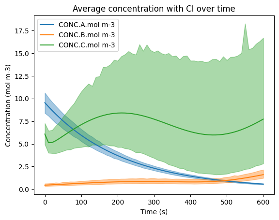
sns.lineplot(data=df_expanded, x='time.s', y='CONC.A.mol m-3', errorbar=('ci', 95), err_kws={'alpha' : 0.4}, label='CONC.A.mol m-3')
sns.lineplot(data=df_expanded, x='time.s', y='CONC.B.mol m-3', errorbar=('ci', 95), err_kws={'alpha' : 0.4}, label='CONC.B.mol m-3')
sns.lineplot(data=df_expanded, x='time.s', y='CONC.C.mol m-3', errorbar=('ci', 95), err_kws={'alpha' : 0.4}, label='CONC.C.mol m-3')
plt.title('Average concentration with CI over time')
plt.ylabel('Concentration (mol m-3)')
plt.xlabel('Time (s)')
plt.legend()
plt.show()

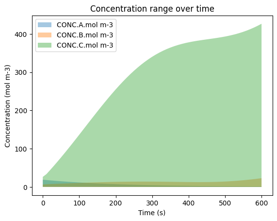
min_y = []
max_y = []
for i in range(0, sim_length + 1, time_step):
        min_y.append({key: np.min(value) for key, value in concentrations_solved[int(i/time_step)].items()})
        max_y.append({key: np.max(value) for key, value in concentrations_solved[int(i/time_step)].items()})
time_x = list(map(float, range(0, sim_length + 1, time_step)))

plt.fill_between(time_x, [y['A'] for y in min_y], [y['A'] for y in max_y], alpha = 0.4, label='CONC.A.mol m-3')
plt.fill_between(time_x, [y['B'] for y in min_y], [y['B'] for y in max_y], alpha = 0.4, label='CONC.B.mol m-3')
plt.fill_between(time_x, [y['C'] for y in min_y], [y['C'] for y in max_y], alpha = 0.4, label='CONC.C.mol m-3')
plt.title('Concentration range over time')
plt.ylabel('Concentration (mol m-3)')
plt.xlabel('Time (s)')
plt.legend()
plt.show()

	time.s	ENV.temperature.K	ENV.pressure.Pa	ENV.air number density.mol m-3	CONC.A.mol m-3	CONC.B.mol m-3	CONC.C.mol m-3
0	0	306.77118255397335	101710.44212531002	39.87647830870052	0.9525640731748064	0.9277350930836727	2.109484498727772
1	0	306.77118255397335	101710.44212531002	39.87647830870052	16.1838357293515	0.14087529981434949	4.964760487510522
2	0	306.77118255397335	101710.44212531002	39.87647830870052	0.6477459211376233	0.9280171925293287	8.81391353397903
3	0	306.77118255397335	101710.44212531002	39.87647830870052	11.150814125867477	0.2986852181763648	3.488685259641938
4	0	306.77118255397335	101710.44212531002	39.87647830870052	1.6547100335371099	0.41897697457943517	2.0460424913055597
...	...	...	...	...	...	...	...
6095	600	306.77118255397335	101710.44212531002	39.87647830870052	0.8619781591486495	1.1052587028684329	2.1882747277796657
6096	600	306.77118255397335	101710.44212531002	39.87647830870052	0.06836507178554663	2.1904066206317956	1.0536360857508953
6097	600	306.77118255397335	101710.44212531002	39.87647830870052	0.4623524932103501	2.0560294025235155	3.7040621977405275
6098	600	306.77118255397335	101710.44212531002	39.87647830870052	0.3261281461119355	1.805009413384805	18.01667944817071
6099	600	306.77118255397335	101710.44212531002	39.87647830870052	0.12717481687495982	2.5985321275364996	1.2225250496271358

6100 rows × 7 columns